
Let’s say you already trained your Machine Learning (ML) model and would like to know if it performs well. In order to do that it is necessary to know and apply the correct metric to evaluate your ML model. This article will give you a brief overview of metrics that can be used for classification & regression models. For more information regarding AI and types of machine learning like classification & regression, check out this article.
Metrics for Classification
Models such as support vector machine (SVM), logistic regression, decision trees, random forest, XGboost, convolutional neural network, recurrent neural network are some of the most popular classification models. To evaluate these models you can use metrics like Accuracy, Precision, Recall or F1 Score. A key concept to understand these metrics is the so-called Confusion Matrix.
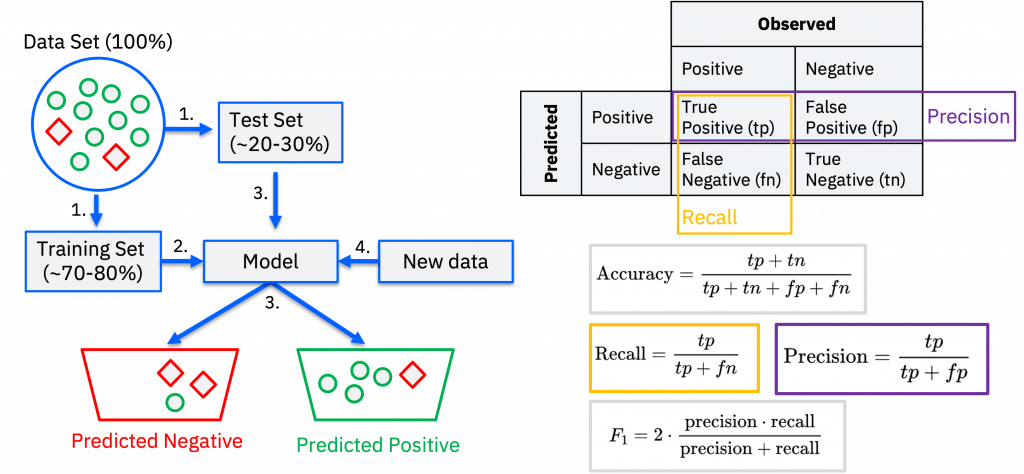
In the picture below you can see on the left-hand side the process of how a binary classification model (only 2 classes like Positive or Negative, true or false, 1 or 0) is trained and tested. In Step 1 the data set (100% of the data) gets split into a training set (~70-80% of the data) and a test set (~20-30% of the data). In Step 2 you can train a model using the training data and in step 3 you can use the model to make predictions using the test data. In a step 4 you could then apply the model to new data, for instance if you use it in production.
On the right hand-side you can see the Confusion Matrix on top and the formulas to calculate Accuracy, Precision, Recall and F1 Score. The Confusion Matrix is a tabular visualization of the model predictions versus the ground-truth or observed, correct values. Each row of the Confusion Matrix represents the instances in a predicted class and each column represents the instances in an actual class. Accuracy considers False Positives (fp) and False Negatives (fn) in the formula, while Recall considers only fn and Precision considers only fp in relation to True Positives (tp). For all 3, a value close to 1, i.e. 100%, is ideal; the larger the fp and fn become, the further the value moves away from 1. One popular metric which combines precision and recall is called F1-score, which is the harmonic mean of precision and recall.
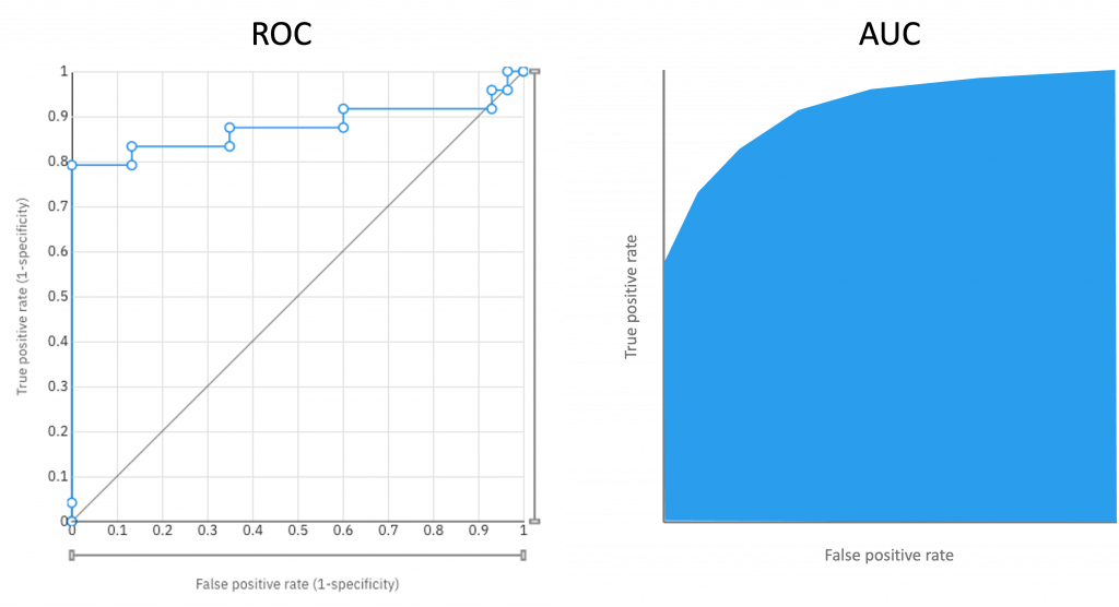
Further metrics for a binary classification are the ROC Curve and AUC.
The receiver operating characteristic (ROC) curve is a graphical representation of the performance of a binary classifier as its threshold is varied. The ROC curve plots the true positive rate (TPR) – a synonym for Recall – against the false positive rate (FPR) at various threshold values. An ideal classifier will have an ROC curve that passes through the upper-left corner (100% TPR and 0% FPR).
A classification models might predict if something is True or False and use a cut-off threshold and if output probability of a prediction is larger than the threshold the prediction will be True, otherwise False. To give an example the model may predict the below samples as True or False depending on the threshold [0.44, 0.61, 0.72, 0.39]:
- threshold / cut-off= 0.5: predicted-labels= [False, True, True ,False] (default threshold)
- threshold / cut-off= 0.25: predicted-labels= [True, True, True, True]
- threshold / cut-off= 0.75: predicted-labels= [False, False, False, False]
As you can see by varying the threshold / cut-off value, we get completely different labels and it would result in a different TPR and FPR rates. The lower the cut-off threshold, the more samples predicted as positive class, i.e. higher true positive rate (TPR) or Recall and also higher false positive rate. Therefore, there is a trade-off between Recall error or FPR.
The area under the ROC curve (AUC) is another commonly used metric to evaluate the performance of a binary classification model. It measures the ability of the model to distinguish between positive and negative examples, and is calculated by computing the area under the ROC curve.
The AUC ranges from 0 to 1, where a value of 0 indicates that the model predictions are 100% wrong, while a value of 1 indicates perfect classification. A higher AUC indicates better performance of the model in terms of discriminating between positive and negative examples.
The AUC is a useful metric because it is insensitive to class imbalance and threshold selection. In other words, it provides a single-number summary of model performance that is not affected by the ratio of positive to negative examples in the dataset, and is not dependent on the choice of threshold for deciding between positive and negative classifications.
In the picture below you can see an 2 separate examples of an receiver operating characteristic (ROC) curve and an area under the ROC curve (AUC).
Metrics for Regression
Models such as linear regression, random forest, XGboost, convolutional neural network, recurrent neural network are some of the most popular regression models. To evaluate these models you can use metrics like Root Mean Square Error (RMSE), Mean Square Error (MSE), Mean Absolute Error (MAE), Median Absolute Error (MedAE), etc. Let’s take a closer look at the RMSE.
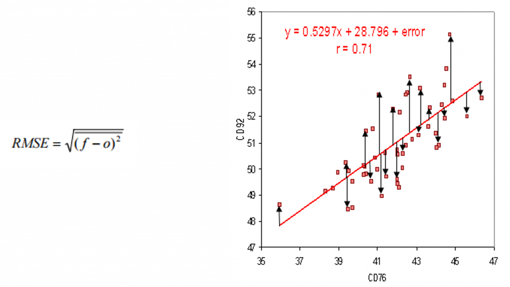
Root Mean Square Error (RMSE) is the standard deviation of the residuals (prediction errors). Residuals are a measure of how far from the regression line data points are; RMSE is a measure of how spread out these residuals are. In other words, it tells you how concentrated the data is around the line of best fit. The lower or closer the RMSE is to 0, the better the model or algorithm.
In the picture below you can see on the left-hand side the formula for RMSE (Where: f = forecasts / expected values or unknown results; o = observed values /known results) and on the right-hand side an example of a regression line, data points and the residuals (distance between data points and line of best fit).
Conclusion
In this article, an introduction to some of the most popular ML metrics used for evaluating the performance of classification and regression models was provided. For further reading and if you want to learn the difference & get started with Artificial Intelligence, Machine Learning & Data Science, continue to this article.